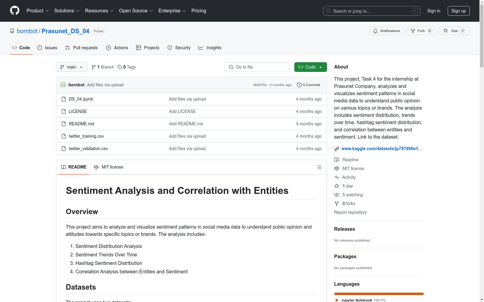
twitter_training.csv 和 twitter_validation.csv

这两个数据集包含推文，每条推文具有以下列：`Tweet ID`（推文标识符）、`Entity`（推文涉及的特定话题或品牌）、`Sentiment`（情感标签，如正面、负面、中性、无关）和`Tweet content`（推文文本内容）。

These two datasets comprise tweets, where each tweet includes the following columns: `Tweet ID` (tweet identifier), `Entity` (specific topic or brand involved in the tweet), `Sentiment` (sentiment labels such as positive, negative, neutral, and irrelevant), and `Tweet content` (text content of the tweet).

原始信息汇总

情感分析与实体相关性

概述

本项目旨在分析和可视化社交媒体数据中的情感模式，以了解公众对特定话题或品牌的意见和态度。分析内容包括：

1. 情感分布分析
2. 情感随时间趋势
3. 标签情感分布
4. 实体与情感的相关性分析

数据集

项目使用两个数据集：

1. twitter_training.csv
2. twitter_validation.csv

两个数据集均包含以下列：

• Tweet ID：推文的标识符。
• Entity：推文涉及的特定话题或品牌。
• Sentiment：情感标签（例如，正面、负面、中性、无关）。
• Tweet content：推文的文本内容。

文件

• DS_04.ipynb：包含情感分析和可视化代码的Jupyter笔记本。
• twitter_training.csv：用于情感分析的训练数据集。
• twitter_validation.csv：用于情感分析的验证数据集。

安装

运行代码需要安装以下Python库：

• pandas
• numpy
• matplotlib
• seaborn

可以使用pip安装所需库： bash pip install pandas numpy matplotlib seaborn

使用

1. 加载数据： 将提供的数据集加载到pandas DataFrame中。 python import pandas as pd

training_data = pd.read_csv(twitter_training.csv) validation_data = pd.read_csv(twitter_validation.csv)

2. 情感分布分析： 使用条形图可视化不同实体的情感分布。 python import matplotlib.pyplot as plt import seaborn as sns

绘制情感分布图

plt.figure(figsize=(12, 6)) sns.countplot(data=training_data, x=Entity, hue=Sentiment, palette=viridis) plt.title(不同实体的情感分布) plt.xticks(rotation=90) plt.show()

3. 情感随时间趋势： 分析情感随时间的变化趋势（需要时间戳数据，此处使用模拟数据演示）。 python import numpy as np

生成模拟时间戳数据

np.random.seed(0) training_data[timestamp] = pd.date_range(start=2021-01-01, periods=len(training_data), freq=H)

按日期和情感分组计数

sentiment_trends = training_data.groupby([training_data[timestamp].dt.date, Sentiment]).size().unstack().fillna(0)

绘制情感随时间趋势图

plt.figure(figsize=(12, 6)) sentiment_trends.plot(kind=line, marker=o) plt.title(情感随时间趋势) plt.xlabel(日期) plt.ylabel(推文数量) plt.legend(title=情感) plt.xticks(rotation=45) plt.show()

4. 标签情感分布： 提取标签并可视化其情感分布。 python import re

从推文内容中提取标签的函数

def extract_hashtags(text): if isinstance(text, str): hashtags = re.findall(r#w+, text) return [hashtag.lower() for hashtag in hashtags] return []

应用函数提取标签

training_data[hashtags] = training_data[Tweet content].apply(extract_hashtags)

展平标签和情感列表

hashtag_sentiment_list = [(hashtag, sentiment) for hashtags, sentiment in zip(training_data[hashtags], training_data[Sentiment]) for hashtag in hashtags]

从列表创建DataFrame

hashtag_sentiment_df = pd.DataFrame(hashtag_sentiment_list, columns=[Hashtag, Sentiment])

按标签和情感分组计数

hashtag_sentiment_counts = hashtag_sentiment_df.groupby([Hashtag, Sentiment]).size().unstack(fill_value=0)

获取总数量前20的标签

top_hashtags = hashtag_sentiment_counts.sum(axis=1).sort_values(ascending=False).head(20).index top_hashtag_sentiment_counts = hashtag_sentiment_counts.loc[top_hashtags]

绘制前20标签的情感分布图

plt.figure(figsize=(14, 8)) top_hashtag_sentiment_counts.plot(kind=bar, stacked=True, colormap=viridis) plt.title(前20标签的情感分布) plt.xlabel(标签) plt.ylabel(推文数量) plt.xticks(rotation=45) plt.legend(title=情感) plt.show()

5. 相关性分析： 检查不同实体与情感之间的关系。 python

创建实体列表

entities = training_data[Entity].unique()

创建实体的二进制矩阵

entity_matrix = pd.DataFrame(0, index=training_data.index, columns=entities)

标记每个推文中实体的存在

for entity in entities: entity_matrix[entity] = training_data[Entity] == entity

将情感标签映射为数值

sentiment_score_mapping = { Positive: 1, Negative: -1, Neutral: 0, Irrelevant: 0 } training_data[sentiment_score] = training_data[Sentiment].map(sentiment_score_mapping)

计算实体存在与情感分数之间的相关性

correlation_matrix = entity_matrix.corrwith(training_data[sentiment_score])

将相关性矩阵转换为DataFrame以便阅读

correlation_df = correlation_matrix.reset_index() correlation_df.columns = [Entity, Correlation]

绘制相关性热图

plt.figure(figsize=(16, 8)) sns.heatmap(correlation_df.set_index(Entity).T, annot=True, cmap=coolwarm, center=0, fmt=".2f", annot_kws={"size": 12}, cbar_kws={label: Correlation}, linewidths=0.5, linecolor=lightgrey) plt.title(实体与情感分数的相关性, fontsize=18) plt.xticks(rotation=45, ha=right, fontsize=14) plt.yticks(fontsize=14) plt.show()

搜集汇总

数据集介绍

构建方式

在构建该数据集时，研究者从Twitter平台采集了大量推文，并对其进行了细致的标注。具体而言，每条推文被赋予了一个唯一的`Tweet ID`，并根据其内容与特定主题或品牌的关系，标注了相应的`Entity`。此外，推文的情绪状态被分类为`Positive`、`Negative`、`Neutral`或`Irrelevant`，并记录在`Sentiment`列中。最后，推文的文本内容被完整地保留在`Tweet content`列中。这种结构化的数据组织方式，为后续的情感分析和相关性研究提供了坚实的基础。

特点

该数据集的显著特点在于其多维度的信息结构和丰富的情感标注。首先，每条推文不仅包含了文本内容，还关联了具体的主题或品牌，这使得研究者能够深入分析特定实体的公众情感反应。其次，情感标签的多样性（包括`Positive`、`Negative`、`Neutral`和`Irrelevant`）为情感分布和趋势分析提供了全面的数据支持。此外，数据集的规模和多样性确保了分析结果的广泛适用性和可靠性。

使用方法

使用该数据集进行分析时，研究者首先需加载`twitter_training.csv`和`twitter_validation.csv`文件，将其转换为pandas DataFrame。随后，可以通过可视化工具如matplotlib和seaborn，对情感分布、趋势和相关性进行深入分析。例如，利用`countplot`函数可以绘制不同实体的情感分布图，而`groupby`和`plot`函数则可用于分析情感随时间的变化趋势。此外，通过正则表达式提取推文中的标签，并结合情感标签进行分布分析，进一步揭示了标签与情感之间的关联。

背景与挑战

背景概述

在社交媒体分析领域，理解和预测公众对特定话题或品牌的态度和情感倾向具有重要意义。`twitter_training.csv`和`twitter_validation.csv`数据集由研究人员创建，旨在通过分析Twitter上的推文来揭示公众情感模式。这些数据集包含了推文的标识符、相关实体、情感标签以及推文内容，为情感分析和实体与情感的相关性研究提供了丰富的数据资源。该数据集的创建不仅推动了社交媒体情感分析技术的发展，也为品牌管理和公共关系研究提供了有力的数据支持。

当前挑战

尽管`twitter_training.csv`和`twitter_validation.csv`数据集为情感分析提供了宝贵的资源，但在其构建和应用过程中仍面临若干挑战。首先，情感标签的准确性依赖于高质量的标注，而社交媒体文本的多样性和复杂性增加了标注的难度。其次，推文内容的实时性和动态变化要求数据集的持续更新和维护。此外，实体与情感的相关性分析需要处理大量的噪声数据和非结构化文本，这对数据处理和分析技术提出了更高的要求。最后，如何有效地从推文中提取和分析情感趋势，以反映公众情感的动态变化，也是一个重要的研究挑战。

常用场景

经典使用场景

在社交媒体情感分析领域，twitter_training.csv 和 twitter_validation.csv 数据集被广泛用于研究公众对特定话题或品牌的情感倾向。通过分析推文内容中的情感标签，研究者可以深入探讨不同实体的情感分布、随时间变化的情感趋势以及与特定话题相关的情感分布。这些分析不仅有助于理解公众舆论的动态变化，还能为品牌管理和市场策略提供有价值的见解。

实际应用

在实际应用中，twitter_training.csv 和 twitter_validation.csv 数据集被广泛用于品牌声誉管理、市场调研和危机公关。企业可以通过分析公众对特定产品的情感反馈，及时调整营销策略，提升品牌形象。此外，政府和非营利组织也可以利用这些数据来监测公众对政策或社会事件的反应，从而制定更有效的沟通策略。

衍生相关工作

基于该数据集，研究者们开发了多种情感分析模型和可视化工具，推动了社交媒体分析领域的发展。例如，一些研究通过结合深度学习技术，提升了情感分类的准确性；另一些研究则开发了实时情感监测系统，用于跟踪公众对重大事件的即时反应。这些衍生工作不仅丰富了情感分析的理论基础，也为实际应用提供了强有力的技术支持。