calabi-yau-data/ws-5d

---
license: cc-by-sa-4.0
pretty_name: Weight Systems Defining Five-Dimensional IP Lattice Polytopes
configs:
- config_name: non-reflexive
data_files:
- split: full
path: non-reflexive/*.parquet
- config_name: reflexive
data_files:
- split: full
path: reflexive/*.parquet
size_categories:
- 100B<n<1T
tags:
- physics
- math
---

# Weight Systems Defining Five-Dimensional IP Lattice Polytopes

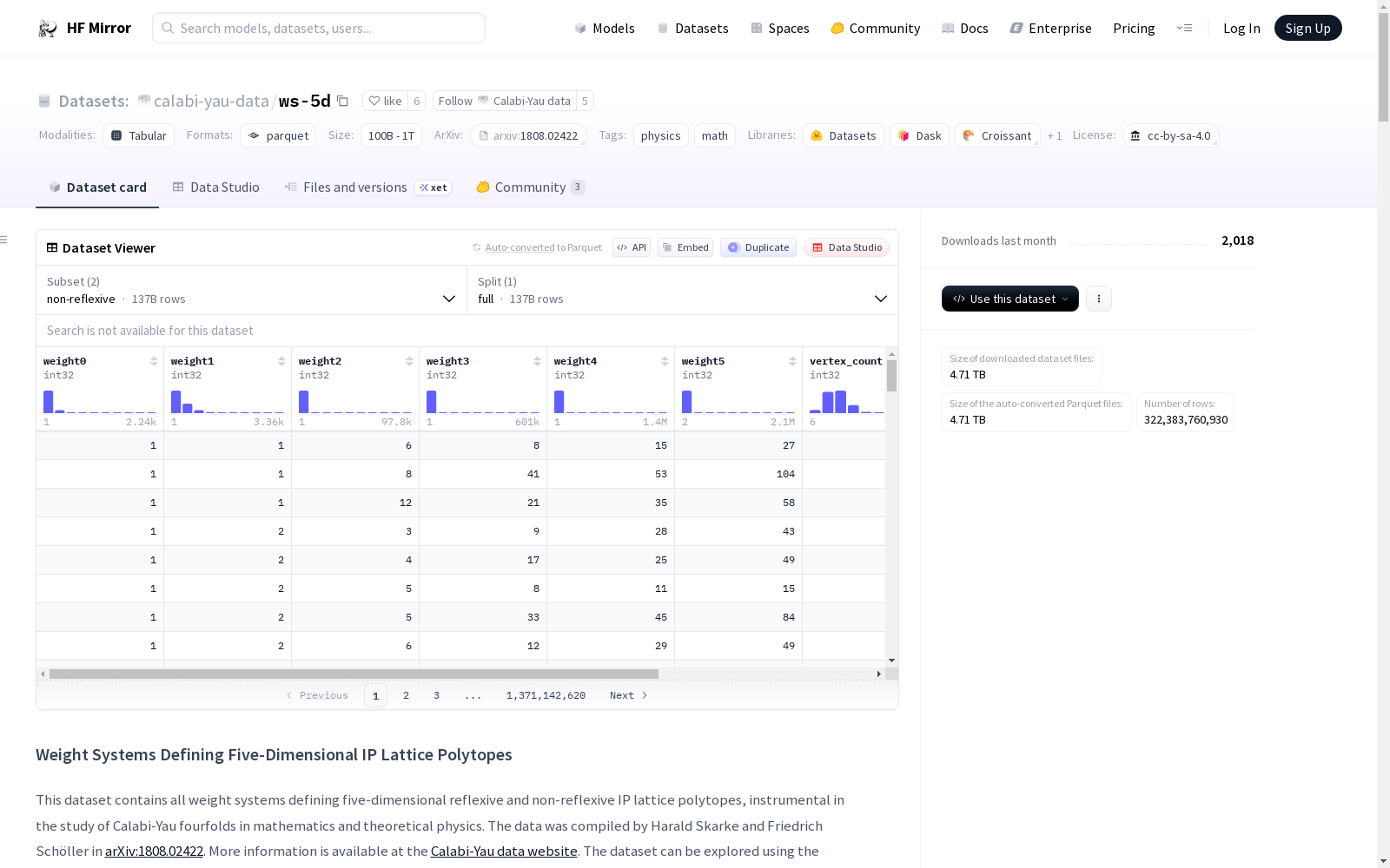
This dataset contains all weight systems defining five-dimensional reflexive and
non-reflexive IP lattice polytopes, instrumental in the study of Calabi-Yau fourfolds in
mathematics and theoretical physics. The data was compiled by Harald Skarke and Friedrich
Schöller in [arXiv:1808.02422](https://arxiv.org/abs/1808.02422). More information is
available at the [Calabi-Yau data website](http://hep.itp.tuwien.ac.at/~kreuzer/CY/). The
dataset can be explored using the [search
frontend](http://rgc.itp.tuwien.ac.at/fourfolds/). See below for a short mathematical
exposition on the construction of polytopes.

Please cite the paper when referencing this dataset:

```
@article{Scholler:2018apc,
author = {Schöller, Friedrich and Skarke, Harald},
title = "{All Weight Systems for Calabi-Yau Fourfolds from Reflexive Polyhedra}",
eprint = "1808.02422",
archivePrefix = "arXiv",
primaryClass = "hep-th",
doi = "10.1007/s00220-019-03331-9",
journal = "Commun. Math. Phys.",
volume = "372",
number = "2",
pages = "657--678",
year = "2019"
}
```

## Dataset Details

The dataset consists of two subsets: weight systems defining reflexive (and therefore IP)
polytopes and weight systems defining non-reflexive IP polytopes. Each subset is split
into 4000 files in Parquet format. Rows within each file are sorted lexicographically by
weights. There are 185,269,499,015 weight systems defining reflexive polytopes and
137,114,261,915 defining non-reflexive polytopes, making a total of 322,383,760,930 IP
weight systems.

Each row in the dataset represents a polytope and contains the six weights defining it,
along with the vertex count, facet count, and lattice point count. The reflexive dataset
also includes the Hodge numbers \\( h^{1,1} \\), \\( h^{1,2} \\), and \\( h^{1,3} \\) of
the corresponding Calabi-Yau manifold, and the lattice point count of the dual polytope.

For any Calabi-Yau fourfold, the Euler characteristic \\( \chi \\) and the Hodge number
\\( h^{2,2} \\) can be derived as follows:

$$ \chi = 48 + 6 (h^{1,1} − h^{1,2} + h^{1,3}) $$

$$ h^{2,2} = 44 + 4 h^{1,1} − 2 h^{1,2} + 4 h^{1,3} $$

This dataset is licensed under the
[CC BY-SA 4.0 license](http://creativecommons.org/licenses/by-sa/4.0/).

### Data Fields

- `weight0` to `weight5`: Weights of the weight system defining the polytope.
- `vertex_count`: Vertex count of the polytope.
- `facet_count`: Facet count of the polytope.
- `point_count`: Lattice point count of the polytope.
- `dual_point_count`: Lattice point count of the dual polytope (only for reflexive
polytopes).
- `h11`: Hodge number \\( h^{1,1} \\) (only for reflexive polytopes).
- `h12`: Hodge number \\( h^{1,2} \\) (only for reflexive polytopes).
- `h13`: Hodge number \\( h^{1,3} \\) (only for reflexive polytopes).

## Usage

The dataset can be used without downloading it entirely, thanks to the streaming
capability of the `datasets` library. The following Python code snippet demonstrates how
to stream the dataset and print the first five rows:

```python
from datasets import load_dataset

dataset = load_dataset("calabi-yau-data/ws-5d", name="reflexive", split="full", streaming=True)

for row in dataset.take(5):
print(row)
```

When cloning the Git repository with Git Large File Storage (LFS), data files are stored
both in the Git LFS storage directory and in the working tree. To avoid occupying double
the disk space, use a filesystem that supports copy-on-write, and run the following
commands to clone the repository:

```bash
# Initialize Git LFS
git lfs install

# Clone the repository without downloading LFS files immediately
GIT_LFS_SKIP_SMUDGE=1 git clone https://huggingface.co/datasets/calabi-yau-data/ws-5d

# Change to the repository directory
cd ws-5d

# Test deduplication (optional)
git lfs dedup --test

# Download the LFS files
git lfs fetch

# Create working tree files as clones of the files in the Git LFS storage directory using
# copy-on-write functionality
git lfs dedup
```

## Construction of Polytopes

This is an introduction to the mathematics involved in the construction of polytopes
relevant to this dataset. For more details and precise definitions, consult the paper
[arXiv:1808.02422](https://arxiv.org/abs/1808.02422) and references therein.

### Polytopes

A polytope is the convex hull of a finite set of points in \\(n\\)-dimensional Euclidean
space, \\(\mathbb{R}^n\\). This means it is the smallest convex shape that contains all
these points. The minimal collection of points that define a particular polytope are its
vertices. Familiar examples of polytopes include triangles and rectangles in two
dimensions, and cubes and octahedra in three dimensions.

A polytope is considered an *IP polytope* (interior point polytope) if the origin of
\\(\mathbb{R}^n\\) is in the interior of the polytope, not on its boundary or outside it.

For any IP polytope \\(\nabla\\), its dual polytope \\(\nabla^*\\) is defined as the set
of points \\(\mathbf{y}\\) satisfying

$$
\mathbf{x} \cdot \mathbf{y}
\ge -1 \quad \text{for all } \mathbf{x} \in \nabla \;.
$$

This relationship is symmetric: the dual of the dual of an IP polytope is the polytope
itself, i.e., \\( \nabla^{**} = \nabla \\).

### Weight Systems

Weight systems provide a means to describe simple polytopes known as *simplices*. A weight
system is a tuple of real numbers. The construction process is outlined as follows:

Consider an \\(n\\)-dimensional simplex in \\(\mathbb{R}^n\\), i.e., a polytope in
\\(\mathbb{R}^n\\) with vertex count \\(n + 1\\) and \\(n\\) of its edges extending in
linearly independent directions. It is possible to position \\(n\\) of its vertices at
arbitrary (linearly independent) locations through a linear transformation. The placement
of the remaining vertex is then determined. Its position is the defining property of the
simplex. To specify the position independently of the applied linear transformation, one
can use the following equation. If \\(\mathbf{v}_0, \mathbf{v}_1, \dots, \mathbf{v}_n\\)
are the vertices of the simplex, this relation fixes one vertex in terms of the other
\\(n\\):

$$ \sum_{i=0}^n q_i \mathbf{v}_i = 0 \;, $$

where \\(q_i\\) is the tuple of real numbers, the weight system.

It is important to note that scaling all weights in a weight system by a common factor
results in an equivalent weight system that defines the same simplex.

The condition that a simplex is an IP simplex is equivalent to the condition that all
weights in its weight system are bigger than zero.

For this dataset, the focus is on a specific construction of lattice polytopes described
in subsequent sections.

### Lattice Polytopes

A lattice polytope is a polytope with vertices at the points of a regular grid, or
lattice. Using linear transformations, any lattice polytope can be transformed so that its
vertices have integer coordinates, hence they are also referred to as integral
polytopes.

The dual of a lattice with points \\(L\\) is the lattice consisting of all points
\\(\mathbf{y}\\) that satisfy

$$
\mathbf{x} \cdot \mathbf{y} \in \mathbb{Z} \quad \text{for all } \mathbf{x} \in L \;.
$$

*Reflexive polytopes* are a specific type of lattice polytope characterized by having a
dual that is also a lattice polytope, with vertices situated on the dual lattice. These
polytopes play a central role in the context of this dataset.

The weights of a lattice polytope are always rational. This characteristic enables the
rescaling of a weight system so that its weights become integers without any common
divisor. This rescaling has been performed in this dataset.

The construction of the lattice polytopes from this dataset works as follows: We start
with the simplex \\(\nabla\\), arising from a weight system as previously described. Then,
we define the polytope \\(\Delta\\) as the convex hull of the intersection of
\\(\nabla^*\\) with the points of the dual lattice. In the context of this dataset, the
polytope \\(\Delta\\) is referred to as ‘the polytope’. Correspondingly,
\\(\Delta^{\!*}\\) is referred to as ‘the dual polytope’. The lattice of \\(\nabla\\) and
\\(\Delta^{\!*}\\) is taken to be the coarsest lattice possible, such that \\(\nabla\\) is
a lattice polytope, i.e., the lattice generated by the vertices of \\(\nabla\\). This
construction is exemplified in the following sections.

A weight system is considered an IP weight system if the corresponding \\(\Delta\\) is an
IP polytope; that is, the origin is within its interior. Since only IP polytopes have
corresponding dual polytopes, this condition is essential for the polytope \\(\Delta\\) to
be classified as reflexive.

### Two Dimensions

In two dimensions, all IP weight systems define reflexive polytopes and every vertex of
\\(\nabla^*\\) lies on the dual lattice, making \\(\Delta\\) and \\(\nabla^*\\) identical.
There are exactly three IP weight systems that define two-dimensional polytopes
(polygons). Each polytope is reflexive and has three vertices and three facets (edges):

| weight system | number of points of \\(\nabla\\) | number of points of \\(\nabla^*\\) |
|--------------:|---------------------------------:|-----------------------------------:|
| (1, 1, 1) | 4 | 10 |
| (1, 1, 2) | 5 | 9 |
| (1, 2, 3) | 7 | 7 |

The polytopes and their duals are depicted below. Lattice points are indicated by dots.
<img src="pictures/ws-2d.png" style="display: block; margin-left: auto; margin-right: auto; width:520px;">

### General Dimension

In higher dimensions, the situation becomes more complex. Not all IP polytopes are
reflexive, and generally, \\(\Delta \neq \nabla^*\\).

This example shows the construction of the three-dimensional polytope \\(\Delta\\) with
weight system (2, 3, 4, 5) and its dual \\(\Delta^{\!*}\\). Lattice points lying on the
polytopes are indicated by dots. \\(\Delta\\) has 7 vertices and 13 lattice points,
\\(\Delta^{\!*}\\) also has 7 vertices, but 16 lattice points.
<img src="pictures/ws-3d-2-3-4-5.png" style="display: block; margin-left: auto; margin-right: auto; width:450px;">

The counts of reflexive single-weight-system polytopes by dimension \\(n\\) are:

| \\(n\\) | reflexive single-weight-system polytopes |
|--------:|-----------------------------------------:|
| 2 | 3 |
| 3 | 95 |
| 4 | 184,026 |
| 5 | (this dataset) 185,269,499,015 |

One should note that distinct weight systems may well lead to the same polytope (we have
not checked how often this occurs). In particular it seems that polytopes with a small
number of lattice points are generated many times.

---
许可证：CC BY-SA 4.0
规范名称：定义五维IP格多面体的权系统
配置项：
- 配置名称：non-reflexive（非自反）
数据文件：
- 拆分方式：full（全量）
路径：non-reflexive/*.parquet
- 配置名称：reflexive（自反）
数据文件：
- 拆分方式：full（全量）
路径：reflexive/*.parquet
规模区间：1000亿 < 数据量 < 1万亿
标签：
- 物理学
- 数学
---
# 定义五维IP格多面体的权系统

本数据集收录了所有定义五维自反与非自反IP格多面体（IP lattice polytope）的权系统，这些多面体在数学与理论物理领域的卡拉比-丘四叶形（Calabi-Yau fourfolds）研究中具有重要作用。本数据集由Harald Skarke与Friedrich Schöller基于[arXiv:1808.02422](https://arxiv.org/abs/1808.02422)汇编完成。更多相关信息可访问[卡拉比-丘数据网站](http://hep.itp.tuwien.ac.at/~kreuzer/CY/)，也可通过[搜索前端工具](http://rgc.itp.tuwien.ac.at/fourfolds/)浏览本数据集。下文将简要介绍多面体构造的相关数学原理。

引用本数据集时，请引用如下论文：

@article{Scholler:2018apc,
author = {Schöller, Friedrich and Skarke, Harald},
title = "{All Weight Systems for Calabi-Yau Fourfolds from Reflexive Polyhedra}",
eprint = "1808.02422",
archivePrefix = "arXiv",
primaryClass = "hep-th",
doi = "10.1007/s00220-019-03331-9",
journal = "Commun. Math. Phys.",
volume = "372",
number = "2",
pages = "657--678",
year = "2019"
}

## 数据集详情

本数据集包含两个子集：定义自反（且为IP）多面体的权系统，以及定义非自反IP多面体的权系统。每个子集均拆分为4000个Parquet格式文件，每个文件内的行按权值的字典序排序。其中，定义自反多面体的权系统共计185,269,499,015组，定义非自反多面体的权系统共计137,114,261,915组，总共有322,383,760,930组IP权系统。

数据集中的每一行对应一个多面体，包含定义该多面体的6个权值，以及顶点数、面数与格点数。自反性子集还包含对应卡拉比-丘流形（Calabi-Yau manifold）的霍奇数（Hodge numbers）( h^{1,1} )、( h^{1,2} )与( h^{1,3} )，以及对偶多面体的格点数。

对于任意卡拉比-丘四叶形，其欧拉示性数( chi )与霍奇数( h^{2,2} )可通过如下公式推导得出：

$$ chi = 48 + 6 (h^{1,1} − h^{1,2} + h^{1,3}) $$

$$ h^{2,2} = 44 + 4 h^{1,1} − 2 h^{1,2} + 4 h^{1,3} $$

本数据集采用[CC BY-SA 4.0许可证](http://creativecommons.org/licenses/by-sa/4.0/)进行授权。

### 数据字段

- `weight0`至`weight5`：定义该多面体的权系统的权值
- `vertex_count`：多面体的顶点数
- `facet_count`：多面体的面数
- `point_count`：多面体的格点数
- `dual_point_count`：对偶多面体的格点数（仅自反多面体子集包含该字段）
- `h11`：霍奇数( h^{1,1} )（仅自反多面体子集包含该字段）
- `h12`：霍奇数( h^{1,2} )（仅自反多面体子集包含该字段）
- `h13`：霍奇数( h^{1,3} )（仅自反多面体子集包含该字段）

## 使用方法

借助`datasets`库的流式读取功能，本数据集无需完整下载即可使用。以下Python代码示例演示了如何流式读取数据集并打印前5行数据：

python
from datasets import load_dataset

dataset = load_dataset("calabi-yau-data/ws-5d", name="reflexive", split="full", streaming=True)

for row in dataset.take(5):
print(row)

当使用Git大文件存储（Git Large File Storage, LFS）克隆仓库时，数据文件会同时存储于Git LFS存储目录与工作树中。为避免占用双倍磁盘空间，请使用支持写时复制（copy-on-write）的文件系统，并执行如下命令克隆仓库：

bash
# 初始化Git LFS
git lfs install

# 克隆仓库且不立即下载LFS文件
GIT_LFS_SKIP_SMUDGE=1 git clone https://huggingface.co/datasets/calabi-yau-data/ws-5d

# 进入仓库目录
cd ws-5d

# 测试重复数据删除（可选）
git lfs dedup --test

# 下载LFS文件
git lfs fetch

# 利用写时复制功能，将工作树文件创建为Git LFS存储目录中文件的克隆
git lfs dedup

## 多面体的构造

本节将介绍与本数据集相关的多面体构造所涉及的数学原理，更详细的内容与精确定义请参阅论文[arXiv:1808.02422](https://arxiv.org/abs/1808.02422)及其参考文献。

### 多面体

多面体是(n)维欧几里得空间(mathbb{R}^n)中有限点集的凸包，即包含该点集的最小凸形。定义一个特定多面体的最小点集即为其顶点。常见的多面体例子包括二维空间中的三角形与矩形，以及三维空间中的立方体与正八面体。

若(mathbb{R}^n)的原点位于多面体内部而非边界或外部，则该多面体被称为**IP多面体**（内点多面体，interior point polytope）。

对于任意IP多面体(
abla)，其对偶多面体(
abla^*)定义为满足对所有(mathbf{x} in
abla)均有( mathbf{x} cdot mathbf{y} ge -1 )的点(mathbf{y})的集合。该对偶关系具有对称性：IP多面体的对偶的对偶即为其本身，即(
abla^{**} =
abla )。

### 权系统

权系统是用于描述一类被称为**单纯形**（simplex）的简单多面体的工具。权系统是一组实数元组，其构造过程如下：

考虑(mathbb{R}^n)中的(n)维单纯形，即顶点数为(n+1)且其中(n)条边沿线性无关方向延伸的多面体。通过线性变换，可将其中(n)个顶点置于任意（线性无关的）位置，剩余顶点的位置便随之确定，该位置是单纯形的核心定义属性。为了在不依赖所采用的线性变换的前提下指定顶点位置，可使用如下等式：若(mathbf{v}_0, mathbf{v}_1, dots, mathbf{v}_n)为单纯形的顶点，则该关系式可通过其余(n)个顶点确定其中一个顶点的位置：
$$ sum_{i=0}^n q_i mathbf{v}_i = 0 ;, $$
其中(q_i)即为构成权系统的实数元组。

需注意的是，将权系统中的所有权值按同一比例缩放，得到的仍是等价的权系统，其定义的单纯形完全相同。

单纯形为IP单纯形的充要条件是其权系统中的所有权值均为正数。

本数据集聚焦于后续章节将介绍的一类格多面体的特定构造方式。

### 格多面体

格多面体是指顶点位于规则网格（即格点）上的多面体。通过线性变换，任意格多面体均可转换为顶点坐标均为整数的形式，因此格多面体也被称为整多面体（integral polytopes）。

格点集合(L)的对偶格是指所有满足对任意(mathbf{x} in L)均有( mathbf{x} cdot mathbf{y} in mathbb{Z} )的点(mathbf{y})构成的格。

**自反多面体**（reflexive polytopes）是一类特殊的格多面体，其对偶仍为格多面体且顶点位于对偶格上。这类多面体在本数据集中处于核心地位。

格多面体的权值始终为有理数，这一特性使得我们可以将权系统按比例缩放，使其权值变为两两互素的整数，本数据集已完成该缩放操作。

本数据集的格多面体构造流程如下：首先基于前文所述的权系统得到单纯形(
abla)，随后将(
abla^*)与对偶格点的交集的凸包定义为多面体(Delta)。在本数据集的语境中，(Delta)被称为“目标多面体”，其对偶(Delta^{!*})被称为“对偶多面体”。我们取(
abla)与(Delta^{!*})所在的格为满足(
abla)为格多面体的最粗格，即由(
abla)的顶点生成的格。后续章节将举例说明该构造过程。

若对应得到的(Delta)为IP多面体（即原点位于其内部），则该权系统被称为IP权系统。由于仅IP多面体存在对应的对偶多面体，该条件是(Delta)被归类为自反多面体的必要条件。

### 二维情形

在二维空间中，所有IP权系统均定义自反多面体，且(
abla^*)的每个顶点都位于对偶格上，因此(Delta)与(
abla^*)完全等价。恰好存在3组IP权系统可定义二维多面体（即多边形），每个多面体均为自反的，且拥有3个顶点与3个面（即边）：

| 权系统 | (
abla)的格点数 | (
abla^*)的格点数 |
|-------:|---------------------:|-----------------------:|
| (1,1,1) | 4 | 10 |
| (1,1,2) | 5 | 9 |
| (1,2,3) | 7 | 7 |

如下所示为这些多面体及其对偶的示意图，格点以圆点标记。<img src="pictures/ws-2d.png" style="display: block; margin-left: auto; margin-right: auto; width:520px;">

### 一般维度情形

在更高维度的情形中，情况会更为复杂。并非所有IP多面体都是自反多面体，且通常情况下(Delta
eq
abla^*)。

本示例展示了权系统为(2,3,4,5)的三维多面体(Delta)及其对偶(Delta^{!*})的构造过程，多面体上的格点以圆点标记。(Delta)拥有7个顶点与13个格点，(Delta^{!*})同样拥有7个顶点，但格点数为16。<img src="pictures/ws-3d-2-3-4-5.png" style="display: block; margin-left: auto; margin-right: auto; width:450px;">

按维度(n)统计的单权系统自反多面体的数量如下：

| 维度(n) | 单权系统自反多面体数量 |
|-----------:|----------------------:|
| 2 | 3 |
| 3 | 95 |
| 4 | 184,026 |
| 5 | （本数据集）185,269,499,015 |

需注意的是，不同的权系统可能会对应同一个多面体（我们尚未统计该情况的发生频率），尤其对于格点数较少的多面体，该重复生成的现象似乎更为明显。

原始信息汇总

五维IP格点多面体权重系统数据集

数据集概述

该数据集包含定义五维自反和非自反IP格点多面体的所有权重系统，这些多面体在数学和理论物理学中对卡拉比-丘四维流形的研究具有重要作用。数据由Harald Skarke和Friedrich Schöller编译，详见arXiv:1808.02422。

数据集详情

数据集分为两个子集：定义自反（因此是IP）多面体的权重系统和定义非自反IP多面体的权重系统。每个子集包含4000个Parquet格式的文件。每个文件中的行按权重字典顺序排序。自反多面体的权重系统有185,269,499,015个，非自反多面体的权重系统有137,114,261,915个，总计322,383,760,930个IP权重系统。

每行数据代表一个多面体，包含定义它的六个权重、顶点数、面数和格点数。自反数据集还包括相应的卡拉比-丘流形的Hodge数 ( h^{1,1} )、 ( h^{1,2} ) 和 ( h^{1,3} )，以及对偶多面体的格点数。

对于任何卡拉比-丘四维流形，Euler特征 ( chi ) 和Hodge数 ( h^{2,2} ) 可以按以下公式计算：

[ chi = 48 + 6 (h^{1,1} − h^{1,2} + h^{1,3}) ]

[ h^{2,2} = 44 + 4 h^{1,1} − 2 h^{1,2} + 4 h^{1,3} ]

数据字段

• weight0 至 weight5：定义多面体的权重系统。
• vertex_count：多面体的顶点数。
• facet_count：多面体的面数。
• point_count：多面体的格点数。
• dual_point_count：对偶多面体的格点数（仅适用于自反多面体）。
• h11：Hodge数 ( h^{1,1} )（仅适用于自反多面体）。
• h12：Hodge数 ( h^{1,2} )（仅适用于自反多面体）。
• h13：Hodge数 ( h^{1,3} )（仅适用于自反多面体）。

使用方法

数据集可以通过datasets库的流式功能进行使用，无需完全下载。以下Python代码片段展示了如何流式读取数据集并打印前五行：

python from datasets import load_dataset

dataset = load_dataset("calabi-yau-data/ws-5d", name="reflexive", split="full", streaming=True)

for row in dataset.take(5): print(row)

数据集构建

数据集中的多面体构建涉及特定的数学过程，详细信息和精确定义请参考arXiv:1808.02422及其参考文献。

搜集汇总

数据集介绍

构建方式

在代数几何与弦理论交叉领域，Calabi-Yau四重形的分类研究依赖于高维格点多面体的系统枚举。本数据集由Harald Skarke与Friedrich Schöller基于arXiv:1808.02422论文构建，通过计算五维IP格点多面体的权重系统，系统生成了反射与非反射两类多面体的完整集合。构建过程始于权重系统定义的单纯形，通过凸包运算与对偶格点交截，逐步导出对应的格点多面体及其对偶结构，最终形成包含超过3220亿条记录的结构化数据。数据以Parquet格式分块存储，各行按权重字典序排列，确保了数学一致性与计算可处理性。

特点

本数据集囊括五维IP格点多面体的全部权重系统，其规模在数学物理数据集中堪称宏大，共包含1852亿反射多面体与1371亿非反射多面体记录。每条记录不仅涵盖定义多面体的六个权重值，还包含顶点数、面数、格点数等几何特征；反射多面体数据进一步提供了对偶多面体的格点数及对应的Calabi-Yau流形的Hodge数h¹¹、h¹²、h¹³。这种设计使得研究者无需重复计算即可直接获取多面体的关键拓扑不变量，并可通过给定公式推导欧拉示性数与h²²等衍生数值，为高维几何与物理模型研究提供了完备的基础数据支持。

使用方法

研究者可通过Hugging Face的datasets库直接流式加载数据集，无需完整下载即可进行高效数据访问。例如，使用Python代码指定反射子集并读取前若干行，即可快速探查数据结构。对于需要本地克隆的场景，数据集支持Git LFS管理，配合写时复制文件系统可避免存储冗余。数据集的官方搜索前端提供了交互式查询界面，便于按几何属性筛选多面体。在理论物理与代数几何研究中，该数据集常用于Calabi-Yau四重形分类、镜像对称性检验以及弦紧化模型的构建，其结构化格式也适合机器学习方法进行模式挖掘与预测建模。

背景与挑战

背景概述

在弦理论与代数几何的交叉领域，Calabi-Yau流形的分类与性质研究始终是核心议题之一，其高维形态的探索对于理解紧化方案与物理对偶性至关重要。数据集'Weight Systems Defining Five-Dimensional IP Lattice Polytopes'由Harald Skarke与Friedrich Schöller于2018年构建，并发表于《Communications in Mathematical Physics》期刊。该数据集系统性地收录了五维自反与非自反IP格点多面体所对应的全部权重系统，旨在为Calabi-Yau四维流形的几何拓扑表征提供完备的计算基础。通过精确枚举超过三千亿个权重系统及其衍生的Hodge数等不变量，该资源极大地推动了高维Calabi-Yau空间的理论图谱绘制，成为数学物理领域连接组合几何与微分几何的桥梁。

当前挑战

该数据集致力于解决高维Calabi-Yau流形系统分类中的组合几何挑战，其核心在于从海量权重系统中精确提取与流形拓扑性质对应的格点多面体。构建过程中的主要困难体现在计算复杂性层面：五维IP多面体的枚举规模达到百亿量级，需设计高效算法以处理整数权重系统的生成、自反性判定及Hodge数计算；同时，数据存储与验证面临严峻压力，需平衡完整性校验与分布式存储的可行性。此外，权重系统到多面体的映射并非一一对应，同一多面体可能被多个权重系统重复生成，这为数据去重与唯一性分析带来了理论上的复杂性。

常用场景

经典使用场景

在代数几何与弦理论领域，Calabi-Yau流形的分类与性质研究始终是核心议题。该数据集通过系统收录五维IP格点多面体的权重系统，为构建Calabi-Yau四重形提供了精确的数学基础。研究者利用这些数据，能够高效地枚举和筛选满足特定几何条件的流形，例如通过Hodge数计算欧拉特征，从而在庞大的解空间中定位具有物理意义的候选对象。这一过程极大地加速了理论模型的构建与验证，成为连接抽象数学结构与具体物理理论的关键桥梁。

解决学术问题

该数据集直接应对了高维Calabi-Yau流形系统化分类的长期挑战。传统方法在枚举四重形时面临组合爆炸问题，而本数据集提供的海量权重系统与多面体数据，使得研究者能够通过算法自动计算Hodge数、对偶多面体点数等关键拓扑不变量。这不仅解决了流形完备性列表的生成难题，还深化了对反射与非反射多面体对应几何结构的理解，为弦紧化、镜对称等前沿理论提供了坚实的数值依据，推动了数学物理交叉领域的定量化研究进程。

衍生相关工作

围绕该数据集衍生的经典工作，主要集中在高维流形分类算法的优化与物理模型的构建。例如，基于数据集的完备性，后续研究深入分析了权重系统与多面体几何的对应关系，提出了更高效的反射多面体生成算法。在物理方面，学者利用数据集枚举的流形，系统探索了四维有效理论中的粒子谱与耦合常数，推动了弦景观的定量化研究。这些工作不仅巩固了数据集在领域内的基石地位，也催生了诸多关于格点多面体组合性质与几何拓扑关联的新颖理论成果。