Uris001/credit-risk-eda

---
license: mit
task_categories:
- tabular-classification
configs:
- config_name: default
data_files:
- split: train
path: data.csv
---
# Credit Risk Analysis — Exploratory Data Analysis (EDA)
<video src="https://huggingface.co/datasets/Uris001/credit-risk-eda/resolve/main/video.mp4" controls width="720"></video>
## 1. Objective
This project identifies the key factors influencing loan default risk through exploratory data analysis. The README focuses on the most informative variables; the full analysis and code are available in the accompanying Google Colab notebook.

## 2. Dataset Overview

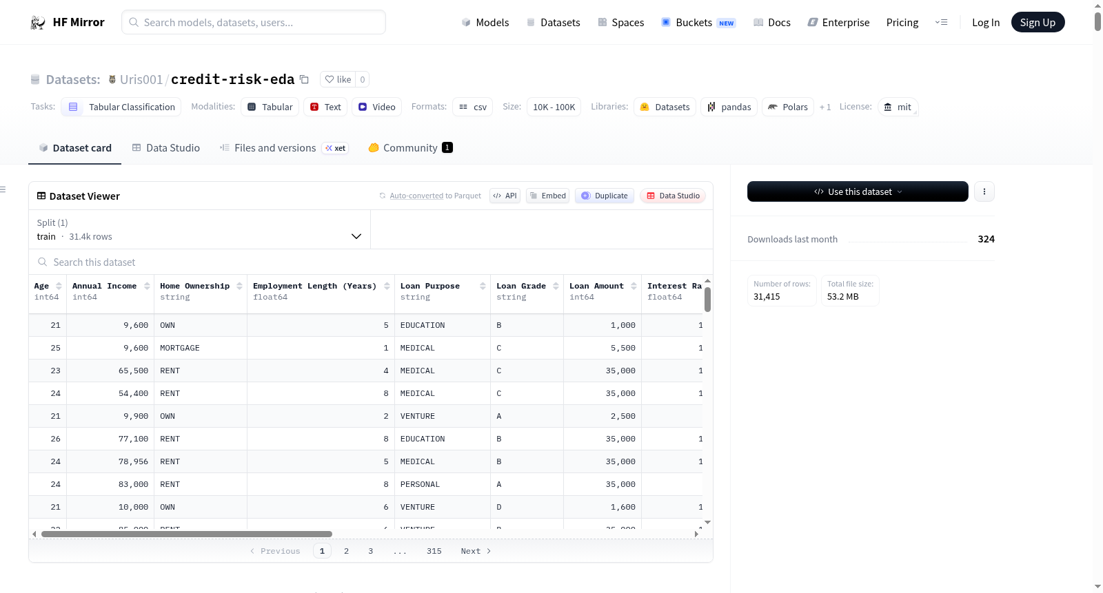
The dataset contains borrower level information used to analyze credit default risk. Each observation represents a single loan application with associated financial, demographic, and behavioral attributes.

* Raw size - Number of observations: 32,581 rows & 12 features
* Clean size - 31,415 rows & 12 original features + 4 engineered groups = 16 total

### Feature Categories:
| Feature | Type | Description |
|----------------|------------|-------------|
| Age | Numeric | Age of the borrower |
| Annual Income | Numeric | Borrower’s yearly income |
| Home Ownership | Categorical| Type of home ownership of the individual: Rent, Mortgage, Own & other |
| Employment Length | Numeric | Years of employment history |
| Loan Purpose | Categorical| Reason for loan |
| Loan Amount | Numeric | Total borrowed amount |
| Interest Rate | Numeric | Rate assigned based on risk. |
| Loan % Income | Numeric | ratio of loan amount to income. |
| Credit History | Numeric | The length of credit history for the individual. |
| Previous Default | Binary | indicator of past default behavior (0 = No, 1 = Yes). |
| Loan Grade | Ordinal | The grade assigned to the loan based on the creditworthiness of the borrower: A (low risk) → G (high risk) |
| Default Status | Binary | Default Status — binary variable (0 = no default, 1 = default): |
| Age Group | Categorical | Age segmented into groups (e.g., 18–25, 26–35, …) |
| Income Group | Categorical | Income divided into quantiles (Very Low → Very High) |
| LTI Group | Categorical | Loan-to-Income ratio grouped into quantiles (Very Low → Very High) |
| Interest Rate Group | Categorical | Interest rate grouped into quantiles (Very Low → Very High) |
#### Target Variable

* Default Status — binary variable (0 = no default, 1 = default):
* 0: Non-default - The borrower successfully repaid the loan as agreed, and there was no default.
* 1: Default - The borrower failed to repay the loan according to the agreed-upon terms and defaulted on the loan.
This variable represents the outcome of the loan and is used to analyze how different borrower and loan characteristics relate to default risk.

### Analytical Notes

- Mix of numerical and categorical variables with skewed distributions (notably income and loan amount)
- Outliers validated against real-world plausibility; extreme but realistic values retained
- Continuous variables segmented into quantile-based groups for interpretability
- Relative measures (e.g., LTI) prioritized over absolute valu

---

## 3. Methodology
The analysis follows a structured and decision driven exploratory data analysis (EDA) pipeline designed to uncover patterns in credit default behavior.

### 3.1 Data Cleaning
#### Column Standardization
Column names were revised to improve clarity and consistency. In addition, categorical values in the Previous Default variable were standardized by replacing abbreviations (“Y”/“N”) with full labels (“Yes”/“No”) to enhance readability and interpretability.

#### Invalid Values Handling
Initial exploratory checks revealed unrealistic values in key variables:
- Ages exceeding 90 years
- Employment length values above realistic working ranges (e.g.,60 years)

These values were removed from the dataset. Given their small proportion and clear inconsistency with real-world constraints, removing these rows ensured data quality without introducing bias or significantly reducing dataset size.

#### Missing Values Treatment
Missing interest rate values were imputed using the within loan grade median, preserving the relationship between loan grade and intrest rate.
Median over mean, robust to skewed financial distributions.

### Small Group Assessment

A systematic scan of all categorical variables was conducted to
identify groups with insufficient sample sizes for reliable estimation.

**Home Ownership — OTHER (n=106)**

The OTHER category was removed from analysis (<0.3% of dataset).Sample size is insufficient for reliable default rate estimation and the category lacks a clear real-world definition.

**Loan Grade — F and G**

Grades F and G were identified as small groups but retained in the analysis. Although limited in size, these grades represent the highest-risk borrower segment and carry meaningful analytical value. Default rate estimates for these grades should be interpreted with caution given the small sample sizes.

---
### 3.2 Duplicates and Outliers
#### Duplicates
A total of 156 duplicate rows were identified and removed to ensure data integrity and avoid bias from repeated observations.

#### Outlier Detection and Treatment
Outliers were identified using boxplots and the IQR method. Invalid values were removed, while extreme but realistic financial observations were retained to preserve dataset variability and reflect real world borrower heterogeneity.

- Invalid outliers (e.g., unrealistic ages and employment durations) were treated as data errors and removed during preprocessing.
- Financial outliers (e.g., Annual Income, Loan Amount, Interest Rate, Credit History Length and Loan to Income ratio) were retained.

Outlier Detection:

#### Rationale
Financial variables naturally exhibit right skewed distributions, driven by a small number of high value observations. These extreme values reflect real world heterogeneity among borrowers rather than errors.
Removing them would eliminate critical information about high income individuals and high risk loan profiles.

Sensitivity analysis was conducted across three binning schemes — quantile, equal-width, and tertile — for each continuous variable analyzed. For LTI and interest rate, the monotonic relationship with default rate is consistent across all three schemes, confirming robustness. For income, equal-width binning produces near-empty upper groups due to severe right skew, making quantile binning the appropriate choice for this variable specifically. The sharp increase in default rate observed in the highest LTI and interest rate groups survives all binning schemes and is interpreted as a genuine nonlinearity rather than a boundary artifact.

---
## 4. Exploratory Data Analysis (EDA)
### Research Question:

What factors are associated with a higher likelihood of loan default?

This is the bigger question that I would like to answer.

### Observation:

The distribution of the target variable shows that approximately 78% of borrowers successfully repay their loans, while around 22% default. This indicates that the dataset is moderately imbalanced, with non default cases being more prevalent.

Despite the imbalance, the proportion of default cases is sufficiently large to allow meaningful analysis of factors influencing credit risk.

---
### Research Question 1:
#### How effectively does loan grade capture borrower default risk?

### Observation:
* Grades A and B comprise ~65% of the dataset; lower grades (E–G) are a small minority.
* Default rates increase monotonically A → G: grades A–C range from 9% → 20%, all at or below the 21.6% baseline.
* A sharp jump from C → D (20% → 59%) marks a structural break, not a gradual transition.
* Grades D–G exhibit default rates from 58% → 98%, far above baseline.
* Sample sizes decline steeply with risk (~10K at A vs. 64 at G), indicating intentional lender risk controls.

### Insight:
Near-perfect separation between low-risk (A–C) and high-risk (D–G) segments.
The C→D threshold suggests the grading system embeds a hard risk boundary, not just a linear scale.
Grade distribution skew (many low-risk, few high-risk) reflects real-world lending behavior lenders limit exposure to high risk borrowers.
### Conclusion:
Loan grade is one of the most informative predictors of default, an aggregated feature that summarizes complex financial and behavioral characteristics into a single well calibrated variable.
### Statistical View:

| Signal | Detail |
|---|---|
| Monotonic risk ladder | Default rises consistently from 10% (A) → 98% (G) |
| Critical threshold C→D | Jump from 20% → 59%; transition from manageable to high risk |
| Grades D–G | Default rates exceed 60%, reaching near-certainty at G |
| Confidence intervals | Tight across all grades, including small samples |
| Sample size decay | ~10K (A) → 64 (G); consistent with intentional risk exposure limits |

---
### Research Question 2:
**Does income group influence default risk?**

**Observation:**
- Mean income ($66.5K) exceeds median ($56K) — high-income outliers pull the average upward.
- Distribution is strongly right-skewed; log transformation yields a near-normal distribution centered at log ≈ 11 (~$60K, consistent with the median).
- The boxplot confirms the signal directly: non-defaulters (green) show a higher and tighter IQR centered at log ≈ 11, while defaulters (red) sit lower with a wider spread — indicating both lower typical income and greater income variability among those who default.
- Both groups contain high-income outliers, explaining the mean–median gap and confirming that the skew is driven by a small number of extreme values, not the general population.
- Raw income alone cannot cleanly separate risk levels — the overlap between the two boxplots is substantial. Quantile-based grouping was applied specifically to overcome this, collapsing noisy continuous values into structured, comparable risk segments.
- After quantile-based grouping (Very Low → Very High), a clear downward trend emerges: Very Low defaults at ~42–45%, Very High at ~8–10%.
- Confidence intervals are tight across all groups, indicating stable estimates.

[](https://cdn-uploads.huggingface.co/production/uploads/69bbf8151e6d7201351aebeb/sF7WINBaL9AyNUWK4Uy7D.png)
[](https://cdn-uploads.huggingface.co/production/uploads/69bbf8151e6d7201351aebeb/-Ao2MEeotd3sPfxUySJ4_.png)

**Insight:**
- Strong inverse relationship between income and default risk — higher-income borrowers are significantly less likely to default.
- The log boxplot makes the income gap tangible, but the IQR overlap between defaulters and non-defaulters confirms that raw income is insufficient as a standalone separator. Grouping converts a noisy signal into an actionable risk gradient — without it, the inverse relationship with default remains statistically visible but practically uninterpretable.
- Despite the clear trend, income alone does not account for relative loan burden — that is captured by LTI.

**Conclusion:**
Income is a meaningful predictor of default risk, but grouping is essential to reveal it. It should be used alongside relative measures (LTI) rather than in isolation.

---
### Research Question 3:
#### Does Loan to Income ratio significantly increase default risk?

**Observation:**
- The scatter plot of income vs. loan amount shows no clean boundary between defaulters and non-defaulters — the two groups are heavily interleaved when using absolute values alone.
- Key signal from median comparison: defaulters carry lower income (40–50K) and higher loan ($10K) vs. non-defaulters (60K+, $8K) — a higher relative burden at the median despite similar absolute loan ranges.
- Typical borrower cluster: income 30K–80K, loan 3K–15K — this is where the majority of risk mass lies, and where the overlap between groups is densest.
- This overlap is precisely why absolute values fail: two borrowers with the same $20K loan look identical until you account for whether one earns $30K and the other $120K.
- After LTI grouping, the hidden structure becomes visible — default rates increase steadily across groups, with the highest LTI group jumping sharply to ~50%+, more than double the lowest group.


#### Insight:
- Default risk is driven by relative financial burden, not absolute values — LTI is the feature that makes this distinction explicit.
- Income acts as a protective factor: higher income shifts borrowers into safer regions even at identical loan amounts, which is invisible in a standard income or loan amount analysis.
- The monotonic increase across LTI groups confirms that as debt burden relative to income grows, so does the probability of default — not just slightly, but in a structured, predictable gradient.
- LTI is a feature engineering outcome: neither income nor loan amount alone contains this signal. The ratio construction is what unlocks it.

#### Conclusion:
LTI is the strongest individual numerical predictor of default (r = 0.38). It resolves the overlap problem in raw financial variables by reframing the question from "how much did they borrow?" to "how much did they borrow relative to what they can sustain?"

---
### Research Question 4:
#### Does a borrower’s past default behavior significantly predict future default risk?

### Observation:
* The dataset is imbalanced: around 82% of borrowers have no prior default, while 18% have defaulted before.
* The bar chart compares default rates between borrowers with and without a history of previous default.
* Despite being the minority, borrowers with a previous default show a much higher default rate (37–38%) compared to those with no history (18%).
* This represents a substantial increase (more than double) in default probability between the two groups.


### Insight:

* Previous default behavior is a strong behavioral signal of future default risk.
* The sharp difference between the two groups indicates that past financial behavior reflects underlying borrower characteristics such as repayment discipline and financial stability.
* Unlike many financial variables that require transformation or grouping, this feature provides a clear and direct separation between risk levels.
* This suggests that historical behavior captures risk factors that may not be fully observable through income or loan characteristics alone.

### Conclusion:

Past default behavior is one of the strongest predictors of future default, reflecting underlying borrower reliability.

### Interaction Analysis

To assess whether previous default predicts risk uniformly, default rates were examined across loan grade, LTI, and income subgroups.


Three distinct patterns emerge:
- **Grade:** Previous default adds minimal incremental signal within grades D–G — grade already absorbs most of the behavioral risk signal (R² = 28.76% between grade and previous default).
- **LTI:** Previous default compounds consistently with debt burden — a ~15–20 percentage point gap persists across all LTI groups, widening at Very High LTI.
- **Income:** Previous default is income-agnostic — even Very High income borrowers with prior defaults face a 23% default rate, nearly 4x higher than counterparts without prior default (6%).

**Implication:** Previous default operates as an independent behavioral signal relative to income and LTI, but is substantially encoded in loan grade. Its marginal contribution in a model that includes grade should be validated — independent value may be limited to segments not well-separated by grade alone.

---
### Research Question 5:
#### Does home ownership status reflect differences in default risk?

### Observation:
* The dataset is dominated by RENT (51%) and MORTGAGE (41%).
* Default rates differ noticeably across groups:
* RENT is around ~31%, the highest levels
* MORTGAGE sits lower at ~12%
* OWN has the lowest default rate at ~7%
* The gap between OWN and RENT is especially large, suggesting meaningful differences between these groups.

### Insight:
* There’s a clear pattern here: borrowers with more stable or secured housing situations tend to default less.
* Owning a home outright is associated with the lowest risk, which likely reflects stronger financial stability and lower ongoing obligations.
* Mortgage holders fall somewhere in the middle — they carry debt, but still show lower risk than renters.
* RENT stands out as the riskiest major group, possibly because it captures borrowers with less financial cushion or less long-term stability.

### Conclusion:
* Home ownership status does provide useful information about default risk, with a clear gradient from OWN (lowest risk) to RENT (highest consistent risk).
* Overall, this feature adds contextual insight, particularly in distinguishing between stable and less stable borrower segments.

### Statistical View:

| Ownership | Share of Dataset | Default Rate | Risk Tier | vs. RENT |
|---|---|---|---|---|
| OWN | ~8% | ~7% | 🟢 Low | 4.4x lower |
| MORTGAGE | ~41% | ~12% | 🟡 Moderate | 2.6x lower |
| RENT | ~51% | ~31% | 🔴 High | Baseline |

---
### Research Question 6:
#### Is interest rate associated with default risk, and does it reflect risk-based pricing?

### Observation:
* The density curves show a clear rightward shift for defaulters, indicating that they are concentrated at higher interest rates.
* Non-defaulters are more concentrated in the lower to mid interest rate range (6–12%), while defaulters peak at higher levels (12–16%).
* The boxplot shows that borrowers who default tend to have higher interest rates on average than those who do not.
* There is noticeable overlap between the groups, but the median and overall distribution shift upward for defaulters.
* When grouping interest rates into quantile based bins, a clear pattern appears:
* Default rates increase steadily from Very Low → High
* The Very High interest rate group shows a sharp jump (~48–50%), significantly above all other groups
* Within-grade analysis confirms that interest rate bands are largely non-overlapping across grades, with within-grade standard deviation of 1% percentage point against a between-grade spread of 13% points.
*

**Endogeneity Finding:**
Subgroup analysis of default rates by interest rate group within each loan grade shows near-flat patterns across all grades with sufficient data. Grade C shows an apparent anomaly but is based on n=71 observations and is excluded from interpretation. Partial correlation between interest rate and default, after removing the grade-mediated component, yields r = −0.04.

**Insight:**
- Interest rate is primarily a pricing output of loan grade, not an independent risk predictor — the raw correlation (r = 0.34) reflects grade's simultaneous effect on both variables.
- Lenders appear to price risk into the loan: higher-risk borrowers receive higher rates, which in turn increases financial burden and may compound default probability.
- The sharp jump in the Very High rate group likely reflects this compounding effect rather than rate as a standalone driver.

**Conclusion:**
Interest rate is strongly associated with default risk but should not be interpreted as causal. It is both a signal of underlying risk (via grade) and a potential contributor to default through increased financial burden. Once grade is controlled for, its independent predictive value is near zero (r = −0.04).

---
## 5. Correlation Structure
## Key Correlations with Default Status

| Variable | Correlation | Direction |
|---|---|---|
| Loan Grade (numeric) | 0.38 | Positive |
| Loan % of Income | 0.38 | Positive |
| Interest Rate | 0.34 | Positive |
| log_income | −0.27 | Negative |
| Annual Income | −0.16 | Negative |

## Redundancy Flags (Multicollinearity)

| Variable Pair | Correlation |
|---|---|
| Interest Rate ↔ Loan Grade | 0.94 |
| Age ↔ Credit History Length | 0.88 |
| Annual Income ↔ log_income | 0.80 |

## Takeaway

The strongest predictors of default are **loan grade, loan-to-income ratio, and interest rate** — all reflecting lender-assessed risk and borrower strain. **log_income (−0.27)** outperforms raw income (−0.16), justifying the log transform. Demographic variables (age, credit history, employment length) show no meaningful linear relationship with default.

---
## 6. Loan Grade as a Mediating Aggregator

Loan grade is assigned by the lender and potentially encodes multiple borrower features. Two analyses were conducted to test this: (1) correlation of each feature with loan grade (R²) to measure encoding, and (2) partial correlation with default after removing the grade-mediated component to isolate independent signal.

---

### Finding 1 — Grade Encodes Almost Nothing Except Behavioral History

| Variable | Correlation with Grade | R² |
|---|---|---|
| Income | −0.006 | ~0% |
| LTI | 0.125 | 1.56% |
| Employment Length | −0.049 | 0.24% |
| Credit History | 0.013 | 0.02% |
| Previous Default | 0.536 | 28.76% |

The grading system in this dataset is primarily driven by behavioral history, not by income, debt burden, or employment stability.

---

### Finding 2 — Most Variables Carry Independent Signal

| Variable | Raw r | Partial r | Independent Signal |
|---|---|---|---|
| LTI | 0.38 | 0.34 | Strong |
| Income | −0.165 | −0.163 | Full |
| Employment Length | −0.086 | −0.068 | Weak |
| Credit History | −0.018 | −0.023 | None |
| Interest Rate | 0.34 | −0.04 | None (fully redundant with grade) |

[](https://cdn-uploads.huggingface.co/production/uploads/69bbf8151e6d7201351aebeb/eXS07tbzv7rgGDsQ0khtJ.png)

---

### Structural Summary

- **Previous Default → Grade → Default** (mediated)
- **LTI → Default** (independent, strong)
- **Income → Default** (independent, full)
- **Employment Length → Default** (independent, weak)
- **Interest Rate → Grade → Default** (fully mediated, redundant)
- **Credit History → Default** (no signal)

Grade, LTI, income, and previous default each contribute distinct, largely non-overlapping information. Grade does not subsume the others and should not replace individual features — except for interest rate, which is fully redundant given grade.

## 7. Final Conclusion

This analysis demonstrates that loan default risk is not driven by isolated financial variables, but rather by the interaction between borrower capacity, loan characteristics, and behavioral history.

Among all features, Loan-to-Income ratio and Loan Grade emerge as the most informative predictors, highlighting the importance of relative financial stress and structured risk segmentation.

Overall, the findings emphasize that effective credit risk assessment requires combining multiple dimensions of borrower information rather than relying on single variable analysis.

These findings highlight the importance of feature engineering in uncovering hidden relationships that are not observable through raw variables alone.

## 8. Limitations

- Target variable is imbalanced (78:22). Standard accuracy is not a valid evaluation metric — precision-recall AUC and confusion matrix analysis with threshold tuning are required before any resampling is considered.
- The analysis is based on observational data and does not establish causality.
- Some variables may contain residual noise despite cleaning.
- Grouping (e.g., LTI bins) simplifies interpretation but may reduce granularity.

## 9. Notebook & Plots

Full analysis with code: [Google Colab](Google_colab_notebook.ipynb)

## 10. Author

Uri Sivan

搜集汇总

数据集介绍

构建方式

在信贷风险分析领域，数据质量直接影响模型预测的可靠性。该数据集基于原始借贷申请记录构建，初始包含32,581条观测和12个特征。通过系统性的数据清洗流程，移除了年龄超过90岁、就业年限异常等不符合现实逻辑的无效记录，并对缺失的利率数据采用同贷款等级中位数进行填补，以保持变量间的内在关联。此外，重复的156条记录被剔除，确保了样本的独立性。最终数据集保留了31,415条有效观测，并衍生出年龄分组、收入分位数、贷款收入比分位数及利率分位数四个特征，形成包含16个特征的结构化表格。

特点

该数据集聚焦于个人信贷违约预测，其核心特点体现在多维度风险信号的集成与结构化处理。特征涵盖借款人的人口统计信息、财务状况、历史行为及贷款条款，既包含年龄、年收入等连续变量，也包含房屋所有权、贷款目的等分类变量。值得注意的是，数据集通过特征工程构建了相对度量指标，如贷款收入比，这比绝对数值更能揭示违约风险的本质。目标变量为二分类的违约状态，样本分布呈现适度不平衡，违约占比约22%，为风险建模提供了充分的正面样本。连续变量经过分位数分组处理，增强了模型的解释性，同时保留了金融数据中典型的有偏分布与极端但合理的观测值，以反映真实世界的异质性。

使用方法

该数据集适用于表格分类任务，主要用于开发与评估信贷违约预测模型。研究者可直接加载数据文件，利用其丰富的特征探索风险驱动因素。建议在建模前，充分理解数据集中已揭示的强信号，如贷款等级与违约率近乎完美的单调关联、贷款收入比的强预测能力，以及历史违约行为的独立信息价值。对于连续变量，可沿用提供的分位数分组，或根据研究目的尝试其他离散化方案。鉴于数据集的适度不平衡，在训练分类模型时可考虑采用适当的采样策略或损失函数进行调整。数据集附带的详尽探索性分析为特征选择与工程提供了坚实基础，有助于构建稳健且可解释的信用评分模型。

背景与挑战

背景概述

在金融科技与风险管理领域，信用风险评估是核心研究议题，旨在通过量化分析预测借款人的违约可能性。credit-risk-eda数据集应运而生，专注于贷款违约风险的探索性数据分析。该数据集由独立研究者或机构构建并发布于HuggingFace平台，其核心研究问题在于识别影响贷款违约的关键因素，如借款人收入、负债比率、信用历史及住房状况等。通过整合超过三万条贷款申请记录，涵盖财务、人口统计与行为等多维度特征，该数据集为开发更精准的信用评分模型提供了实证基础，对推动普惠金融和风险定价的智能化发展具有显著影响力。

当前挑战

该数据集致力于解决信用风险评估中的核心挑战，即如何在高度不平衡的样本中（违约率约22%）准确识别高风险借款人，并克服特征间复杂的非线性关系与交互效应。构建过程中面临多重挑战：原始数据包含异常值（如超高龄或不切实际的就业年限）与缺失值，需通过严谨的清洗流程（如基于贷款等级的中位数插补）以确保数据质量；同时，财务变量（如收入与贷款金额）呈现严重右偏分布，要求采用分位数分组等工程化方法以揭示风险梯度，并保留反映真实世界异质性的极端值。此外，小样本类别（如高风险贷款等级F与G）的处理需平衡信息保留与统计可靠性，增加了分析复杂度。

常用场景

经典使用场景

在金融风险管理领域，信用风险预测模型构建是该数据集最经典的应用场景。通过对包含借款人年龄、收入、贷款目的、历史违约记录等多维度特征的结构化数据进行分析，研究人员能够训练监督学习分类器，如逻辑回归、梯度提升决策树等，以精准预测贷款违约概率。该数据集经过精心清洗与特征工程，特别引入了贷款收入比等衍生变量，使得模型能够捕捉借款人偿债能力的相对性，而非仅依赖绝对值，从而提升风险评估的区分度与稳健性。

解决学术问题

该数据集有效解决了信用评分模型中特征重要性与交互效应识别的核心学术问题。通过系统性的探索性数据分析，它揭示了贷款等级与违约率之间的单调阶梯关系，以及贷款收入比作为最强数值预测因子的统计显著性。这些发现挑战了传统模型中孤立看待绝对财务指标的局限，推动了学术界对相对债务负担与历史行为信号在风险建模中协同作用的理解，为构建更透明、可解释的信用评估理论框架提供了实证基础。

衍生相关工作

围绕该数据集衍生的经典研究工作主要集中在机器学习模型的可解释性与公平性探索。例如，研究者利用SHAP或LIME等解释性工具，深入剖析了贷款等级、收入分组等特征对模型决策的贡献度，促进了复杂模型在合规领域的应用。此外，针对数据中存在的类别不平衡与潜在偏见，后续工作发展了重采样、代价敏感学习等算法，以减轻对少数高风险群体的误判，推动了负责任人工智能在金融风控中的实践。