Isomorph2026/isomorph-supply-chain-sample
收藏资源简介:
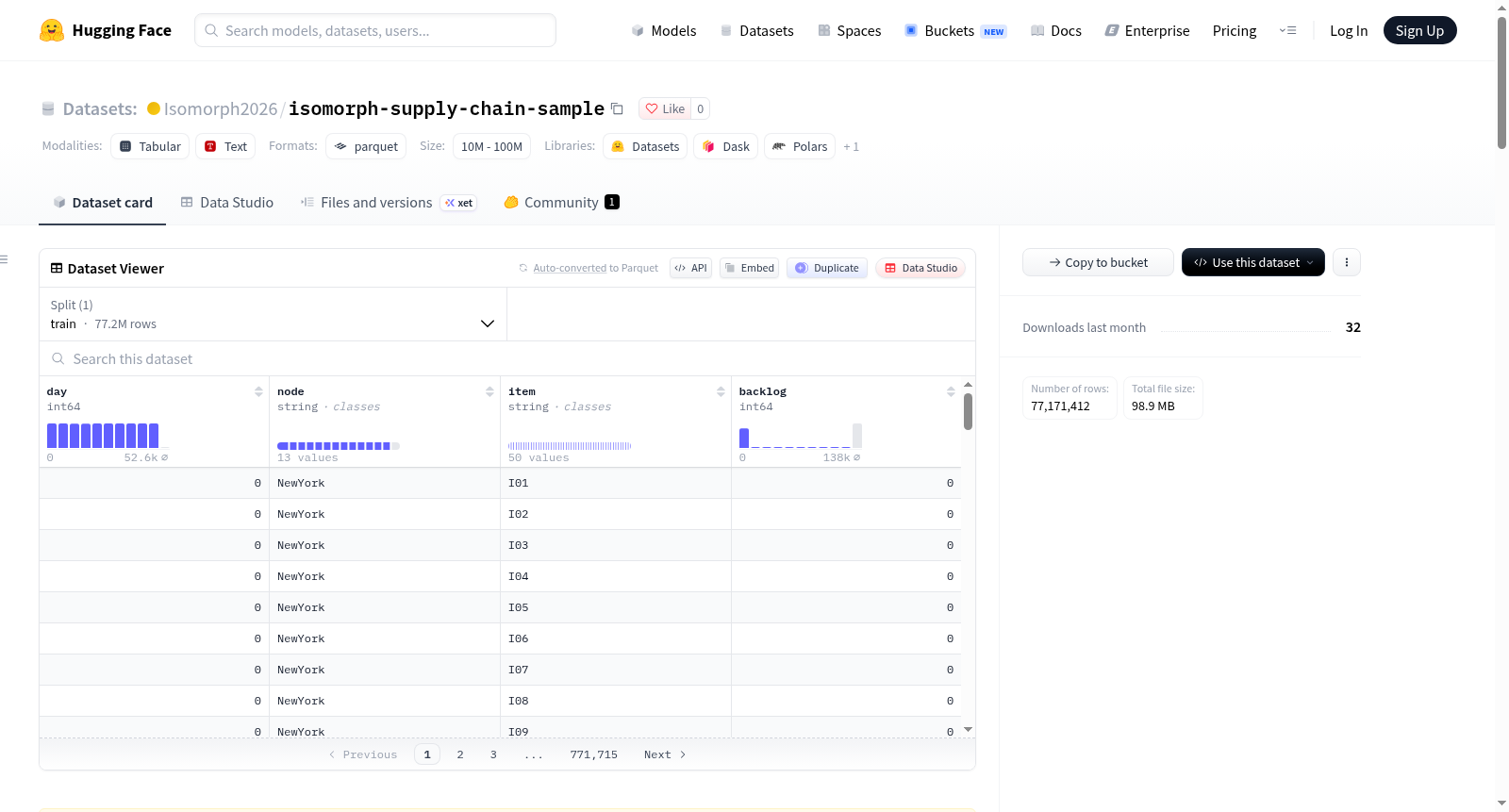
# ISOMORPH Sample A single-rollout subset of the ISOMORPH release, intended for users who want to inspect file formats and run loaders before pulling the full dataset. We release multivariate logistics time-series data generated by a digital-twin (DT) simulator of a multi-echelon supply chain with an explicit routing network, with the underlying dynamics formulated as a Markov chain. ## Overview The simulator advances a directed routing graph of factories, intermediate warehouses, and a customer-facing destination forward in discrete time. At each step, random Poisson customer demand arrives at the destination, is served from on-hand stock, and triggers replenishment along the network. The network is a directed graph $G=(\mathcal{N},\mathcal{E})$ with three node roles (factories, warehouses, destination), integer per-edge transit times $\tau_e$, and per-step volume capacities $K_e V_e$; Dijkstra's algorithm routes every shipment. The dynamics form a Markov chain $\xi_{t+1} = \Psi(\xi_t, y_t, L_t)$, where $\Psi$ is a deterministic transition map and $(y_t, L_t)$ are the only random inputs (Poisson customer demand and Gaussian source lead times). The demand intensity is a five-component sum: yearly seasonality, weekly seasonality, AR(1) drift, per-item bursts, and a shared macro shock that lifts every item's intensity simultaneously. The state vector $\xi_t$ records on-hand stock, backlog, outstanding orders, in-transit shipments, and a smoothed demand estimate at every location for every item. The released rollout runs on a 13-node US topology (3 sources, 9 warehouses across 5 tiers, NYC destination). ## Contents | Item | Notes | |------------------|-----------------------------------------------------------| | `manifest.csv` | One row, the baseline `output_item50` rollout | | `output_item50/` | Rollout directory; see File schema below | ## Rollout summary - Family: `baseline` - Catalogue size C = 50 items - Horizon T = 52,560 days - Seed: 2025 - All knobs at simulator defaults; see `manifest.csv` for exact values - Approximate on-disk size: ~1.9 GB ## Manifest schema `manifest.csv` has one row per rollout (just one in this sample) and the following columns: | Column | Meaning | |------------------------|-------------------------------------------------------------| | `rollout` | Rollout name (matches the directory under this variant) | | `family` | One of `baseline`, `mixture`, `uq` | | `scenario` | Scenario label within the family | | `n_items` | Catalogue size C (50 or 200) | | `seed` | RNG seed (2025 here) | | `horizon` | Length T in days (52,560 here) | | `path` | Relative path to the rollout directory inside this variant | | `phi_lo`, `phi_hi` | AR(1) coefficient bounds for the demand process | | `shock_count_scale` | Multiplier on per-day shock count | | `shock_height_scale` | Multiplier on shock magnitude | | `burst_rate_scale` | Multiplier on burst arrival rate | | `burst_height_scale` | Multiplier on burst magnitude | | `containers_scale` | Multiplier on edge container counts (capacity) | | `ss_scale` | Multiplier on safety-stock thresholds | | `leadtime_scale` | Multiplier on edge lead times | Three additional simulator knobs are held fixed and therefore omitted from the manifest: `seasonal_scale = 1.0`, `base_lambda_lo = 80.0`, `base_lambda_hi = 250.0`. The exact values are still recorded in `output_item50/scenario.json`. ## File schema Directory layout: ``` isomorph_sample/ ├── manifest.csv ├── README.md ├── LICENSE └── output_item50/ ├── daily_records.parquet ├── shipments.parquet ├── service_summary.parquet ├── inventory_history.parquet ├── backlog_history.parquet ├── intransit_history.parquet ├── demand_signals.npy ├── demand_signals_cols.txt ├── scenario.json ├── edge_list.parquet ├── edge_utilisation.npy └── edge_saturation.npy ``` `T` is the run horizon (52,560 for the released rollout), `C` is the catalogue size (50), and `E` is the number of edges in the network. | File | Shape / format | Contents | |----------------------------|-------------------------------|----------------------------------------------------------------------| | `daily_records.parquet` | rows: T x C | Per-day, per-item demand and service: `day, item, demand, served_from_stock, new_backlog_today, dest_on_hand_end_before_ship, dest_backlog_end_before_ship` | | `shipments.parquet` | rows: variable | One row per shipment: `day, arrival_day, from, to, item, units, path_nodes, edge_times` | | `service_summary.parquet` | rows: C | Per-item totals: `total_demand, served_from_stock, new_backlog_added, fill_rate_stock_only` | | `inventory_history.parquet`| rows: T | On-hand inventory over time | | `backlog_history.parquet` | rows: T | Backlog over time | | `intransit_history.parquet`| rows: T | In-transit units over time | | `demand_signals.npy` | array: T x C, float | Item-level demand series (same content as the `demand` column of `daily_records.csv`, dense form) | | `demand_signals_cols.txt` | text | Item IDs in column order of `demand_signals.npy` | | `scenario.json` | JSON | Exact CLI knobs used to produce the rollout | | `edge_list.parquet` | rows: E | Edge metadata: `edge_id, from, to, travel_time_days, container_volume, num_containers, cap_per_day` | | `edge_utilisation.npy` | array: T x E, float | Per-edge fractional utilisation | | `edge_saturation.npy` | array: T x E, float | Per-edge fractional saturation (cap-relative throughput) | ## Quick load ```python import pandas as pd import numpy as np manifest = pd.read_csv("manifest.csv") row = manifest.iloc[0] X = np.load(f"{row.path}/demand_signals.npy") # T x C cols = open(f"{row.path}/demand_signals_cols.txt").read().strip().split(",") records = pd.read_parquet(f"{row.path}/daily_records.parquet") ``` ## Next step For the full benchmark (49 rollouts including mixture sweeps and 20 LHS UQ perturbations), see `../isomorph_full/`. ## Licence CC-BY-4.0 (see `LICENSE`).
ISOMORPH Sample is a single-rollout subset of the ISOMORPH release, intended for users who want to inspect file formats and run loaders before pulling the full dataset. It contains multivariate logistics time-series data generated by a digital-twin simulator of a multi-echelon supply chain with an explicit routing network, formulated as a Markov chain. The simulator advances a directed routing graph of factories, warehouses, and a destination in discrete time, with random Poisson customer demand and Gaussian source lead times as random inputs. Demand intensity is a five-component sum: yearly seasonality, weekly seasonality, AR(1) drift, per-item bursts, and a shared macro shock. The state vector records on-hand stock, backlog, outstanding orders, in-transit shipments, and a smoothed demand estimate for every item at every location. The released rollout runs on a 13-node US topology (3 sources, 9 warehouses across 5 tiers, NYC destination), with parameters: family baseline, catalogue size 50 items, horizon 52,560 days, seed 2025, and approximate on-disk size ~1.9 GB.