convective_envelope_rsg

This Dataset is part of [The Well Collection](https://huggingface.co/papers/2412.00568).

# How To Load from HuggingFace Hub

1. Be sure to have `the_well` installed (`pip install the_well`)
2. Use the `WellDataModule` to retrieve data as follows:

```python
from the_well.data import WellDataModule

# The following line may take a couple of minutes to instantiate the datamodule
datamodule = WellDataModule(
"hf://datasets/polymathic-ai/",
"convective_envelope_rsg",
)
train_dataloader = datamodule.train_dataloader()

for batch in dataloader:
# Process training batch
...
```

# Red Supergiant Convective Envelope

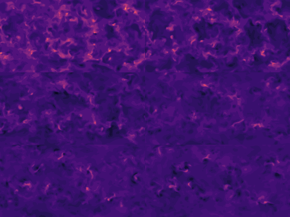
**One line description of the data:** 3D radiation hydrodynamic simulations of the convective envelope of red supergiant stars.

**Longer description of the data:** Massive stars evolve into red supergiants, which have large radii and luminosities, and low-density, turbulent, convective envelopes. These simulations model the (inherently 3D) convective properties and gives insight into the progenitors of supernovae explosions.

**Associated paper**: [Paper](https://iopscience.iop.org/article/10.3847/1538-4357/ac5ab3).

**Domain experts**: [Yan-Fei Jiang](https://jiangyanfei1986.wixsite.com/yanfei-homepage) (CCA, Flatiron Institute), [Jared Goldberg](https://jaredagoldberg.wordpress.com/) (CCA, Flatiron Institute), [Jeff Shen](https://jshen.net) (Princeton University).

**Code or software used to generate the data**: [Athena++](https://www.athena-astro.app/).

**Equations**

$$
\begin{align*}
\frac{\partial\rho}{\partial t}+\mathbf{\nabla}\cdot(\rho\mathbf{v})&=0\\
\frac{\partial(\rho\mathbf{v})}{\partial t}+\mathbf{\nabla}\cdot({\rho\mathbf{v}\mathbf{v}+{{\sf P_{\rm gas}}}}) &=-\mathbf{G}_r-\rho\mathbf{\nabla}\Phi \\
\frac{\partial{E}}{\partial t}+\mathbf{\nabla}\cdot\left[(E+ P_{\rm gas})\mathbf{v}\right] &= -c G^0_r -\rho\mathbf{v}\cdot\mathbf{\nabla}\Phi\\
\frac{\partial I}{\partial t}+c\mathbf{n}\cdot\mathbf{\nabla} I &= S(I,\mathbf{n})
\end{align*}
$$

where

- \\(\rho\\) = gas density.
- \\(\mathbf{v}\\) = flow velocity.
- \\({\sf P_{\rm gas}}\\) = gas pressure tensor.
- \\(P_{\rm gas}\\) = gas pressure scalar.
- \\(E\\) = total gas energy density: \\(E = E_g + \rho v^2 / 2\\), where \\(E_g = 3 P_{\rm gas} / 2\\) = gas internal energy density.
- \\(G^0_r\\) and \\(\mathbf{G}_r\\) = time-like and space-like components of the radiation four-force.
- \\(I\\) = frequency integrated intensity, which is a function of time, spatial coordinate, and photon propagation direction \\(\mathbf{n}\\).
- \\(\mathbf{n}\\) = photon propagation direction.


| Dataset | FNO | TFNO | Unet | CNextU-net |
| :-----------------------: | :--: | :-------------: | :--: | :--------: |
| `convective_envelope_rsg` | \\(\mathbf{0.0269}\\) | 0.0283 | 0.0555 | 0.0799 |

Table: VRMSE metrics on test sets (lower is better). Best results are shown in bold. VRMSE is scaled such that predicting the mean value of the target field results in a score of 1.

## About the data

**Dimension of discretized data:** 100 time-steps of 256 \\(\times\\) 128 \\(\times\\) 256 images per trajectory.

**Fields available in the data:** energy (scalar field), density (scalar field), pressure (scalar field), velocity (vector field).

**Number of trajectories:** 29 (they are cuts of one long trajectory, long trajectory available on demand).

**Estimated size of the ensemble of all simulations:** 570 GB.

**Grid type:** spherical coordinates, uniform in \\((\log r, \theta,\phi)\\). Simulations are done for a portion of a sphere (not the whole sphere), so the simulation volume is like a spherical cake slice.

**Initial and boundary conditions:** The temperature at the inner boundary (IB) is first set to equal that of the appropriate radius coordinate in the MESA (1D) model ( \\(400\~R_\odot\\) and \\(300\~R_\odot\\)) and the density selected to approximately recover the initial total mass of the star in the simulation ( \\(15.4\~M_\odot\\) and \\(14\~M_\odot\\)).
Between \\(300\~R_\odot\\) and \\(400\~R_\odot\\), the initial profile is constructed with the radiative luminosity to be \\(10^5\~L_\odot\\), and this is kept fixed in the IB.

**Simulation time-step:** ~2 days.

**Data are stored separated by ( \\(\Delta t\\)):** units here are sort of arbitrary, \\(\Delta t= 8\\).

**Total time range ( \\(t_{min}\\) to \\(t_{max}\\)):** \\(t_{min} = 2\\), \\(t_{max} = 23402\\) (arbitrary).

**Spatial domain size:** \\(R\\) from \\(300-6700~{\rm R_\odot}\\), θ from \\(π/4−3π/4\\) and \\(\phi\\) from \\(0−π\\), with \\(δr/r ≈ 0.01\\).

**Set of coefficients or non-dimensional parameters evaluated:**

| Simulation | radius of inner boundary \\(R_{IB}/R_\odot\\) | radius of outer boundary \\(R_{OB}/R_\odot\\) | heat source | resolution (r × θ × \\(\phi\\)) | duration | core mass \\(mc/M_\odot\\) | final mass \\(M_{\rm final}/M_\odot\\) |
| ------------------------------------------------ | ----------------------------------------- | ----------------------------------------- | ----------- | --------------------------- | --------- | --------------------- | ---------------------------------- |
| Whole simulation (to obtain the 29 trajectories) | 300 | 6700 | fixed L | 256 × 128 × 256 | 5766 days | 10.79 | 12.9 |

**Approximate time to generate the data:** 2 months on 80 nodes, or approximately 10 million CPU hours.

**Hardware used to generate the data:** 80x NASA Pleiades Skylake CPU nodes.

**Additional information about the simulation:** The radial extent of the simulation domain extends from \\(300~{\rm R_\odot}\\) at the simulation inner boundary to \\(6700~{\rm R_\odot}\\) at the simulation outer boundary, with logarithmic cell spacing in radius. The typical radius of the photosphere (or "surface") of the star is between \\(\approx 800 - 1000 ~{\rm R_\odot}\\), fluctuating in space and time. Convection develops only at locations inside the star, within the first hundred radial zones or so. Some material from the star occasionally reaches larger radial distances.
Outside of the stellar photosphere ("surface"), a density floor is set at \\( \approx 10^{-16} g/cm^3\\), and the material far outside the stellar photosphere generally reflects the infalling motion of gas and density floor material with very little mass, perturbed by the activity of the stellar surface. Additionally, because the temperature and density is very low, the opacities are not well-characterized in this material. So, while the RHD equations are still solved in this region of the simulation domain, one should not interpret things outside \\(\approx 1500 R_\odot\\) as physically meaningful.

## What is interesting and challenging about the data:

**What phenomena of physical interest are captured in the data:** turbulence and convection (inherently 3D processes), variability. Note that the stellar surface only extends out to roughly 1000 \\(R_\odot\\), inside of which the interesting physics occurs.

**How to evaluate a new simulator operating in this space:** can it predict behaviour of simulation in convective steady-state, given only a few snapshots at the beginning of the simulation? can it properly model convection and turbulence?

**Caveats:** complicated geometry, size of a slice in R varies with R (think of this as a slice of cake, where the parts of the slice closer to the outside have more area/volume than the inner parts), simulation reaches convective steady-state at some point and no longer "evolves".

Please cite the associated paper if you use this data in your research:

```
@article{goldberg2022numerical,
title={Numerical simulations of convective three-dimensional red supergiant envelopes},
author={Goldberg, Jared A and Jiang, Yan-Fei and Bildsten, Lars},
journal={The Astrophysical Journal},
volume={929},
number={2},
pages={156},
year={2022},
publisher={IOP Publishing}
}
```

本数据集隶属于[The Well Collection](https://huggingface.co/papers/2412.00568)。

# 从HuggingFace Hub加载数据集

1. 确保已安装`the_well`包（执行`pip install the_well`）
2. 使用`WellDataModule`检索数据，示例代码如下：

python
from the_well.data import WellDataModule

# 以下实例化datamodule可能需要数分钟
datamodule = WellDataModule(
"hf://datasets/polymathic-ai/",
"convective_envelope_rsg",
)
train_dataloader = datamodule.train_dataloader()

for batch in dataloader:
# 处理训练批次
...

# 红超巨星对流包层

**数据单行简介：** 红超巨星恒星对流包层的三维辐射流体动力学模拟。

**数据详细简介：** 大质量恒星演化至红超巨星阶段后，会拥有超大半径与光度，同时包裹着低密度、湍流且处于对流状态的包层。本系列模拟对这类对流的固有三维特性进行建模，可为超新星爆发前身星的研究提供洞察。

**关联论文：** [论文](https://iopscience.iop.org/article/10.3847/1538-4357/ac5ab3)。

**领域专家：** [江燕飞（Yan-Fei Jiang）](https://jiangyanfei1986.wixsite.com/yanfei-homepage)（CCA，Flatiron研究所）、[Jared Goldberg](https://jaredagoldberg.wordpress.com/)（CCA，Flatiron研究所）、[Jeff Shen](https://jshen.net)（普林斯顿大学）。

**生成数据所用代码与软件：** [Athena++](https://www.athena-astro.app/)。

**控制方程**

$$
\begin{align*}
\frac{\partial\rho}{\partial t}+\mathbf{\nabla}\cdot(\rho\mathbf{v})&=0\\
\frac{\partial(\rho\mathbf{v})}{\partial t}+\mathbf{\nabla}\cdot({\rho\mathbf{v}\mathbf{v}+{{\sf P_{\rm gas}}}}) &= -\mathbf{G}_r-\rho\mathbf{\nabla}\Phi \\
\frac{\partial{E}}{\partial t}+\mathbf{\nabla}\cdot\left[(E+ P_{\rm gas})\mathbf{v}\right] &= -c G^0_r -\rho\mathbf{v}\cdot\mathbf{\nabla}\Phi \\
\frac{\partial I}{\partial t}+c\mathbf{n}\cdot\mathbf{\nabla} I &= S(I,\mathbf{n})
\end{align*}
$$

其中：
- (\rho) = 气体密度
- (\mathbf{v}) = 流场速度
- ({\sf P_{\rm gas}}) = 气体压强张量
- (P_{\rm gas}) = 气体压强标量
- (E) = 气体总能量密度：(E = E_g + \rho v^2 / 2)，其中(E_g = 3 P_{\rm gas} / 2)为气体内能密度
- (G^0_r)与(\mathbf{G}_r) = 辐射四维力的类时与类空分量
- (I) = 频率积分强度，是时间、空间坐标与光子传播方向(\mathbf{n})的函数
- (\mathbf{n}) = 光子传播方向


| 数据集名称 | FNO | TFNO | Unet | CNextU-net |
| :-----------------------: | :--: | :-------------: | :--: | :--------: |
| `convective_envelope_rsg` | $\mathbf{0.0269}$ | 0.0283 | 0.0555 | 0.0799 |

**表：测试集上的VRMSE指标（数值越低效果越好），最优结果以粗体标注。VRMSE已进行归一化处理，当预测目标场的均值时，得分为1。**

## 数据集详情

**数据离散化维度：** 每条轨迹包含100个时间步，每个时间步对应尺寸为256 × 128 × 256的三维图像。

**数据包含的物理场：** 能量（标量场）、密度（标量场）、压强（标量场）与速度（矢量场）。

**轨迹总数：** 29条（这些轨迹均来自一条长轨迹的分段，完整长轨迹可按需获取）。

**全部模拟集合的预估总大小：** 570 GB。

**网格类型：** 采用球坐标系，在\((\log r, \theta,\phi)\)方向上均一划分。模拟仅覆盖部分球面区域（非完整球面），因此模拟体积类似一块球形蛋糕切片。

**初始与边界条件：** 内边界（IB）的温度首先设置为与MESA（一维）模型中对应半径处的温度一致（分别为400(R_\odot)与300(R_\odot)），同时调整密度以近似匹配模拟中恒星的初始总质量（分别为15.4(M_\odot)与14(M_\odot)）。在300(R_\odot)至400(R_\odot)区间内，初始剖面通过辐射光度构建为(10^5~L_\odot)，且该值在内边界处保持固定。

**模拟时间步长：** 约2天。

**数据存储间隔：** 数据按时间步长间隔\(\Delta t\)存储：此处单位为任意约定单位，\(\Delta t= 8\)。

**总时间范围：** (t_{min} = 2)，(t_{max} = 23402)（单位为任意约定单位）。

**空间域范围：** 径向半径(R)取值为300–6700({\rm R_\odot})，极角(\theta)取值为\(\pi/4−3\pi/4\)，方位角(\phi)取值为0−\(\pi\)，且满足\(\delta r/r ≈ 0.01\)。

**评估所用的系数与无量纲参数集合：**

| 模拟设置 | 内边界半径 (R_{IB}/R_\odot) | 外边界半径 (R_{OB}/R_\odot) | 热源项 | 空间分辨率 (r × θ × (\phi)) | 模拟时长 | 核心质量 (mc/M_\odot) | 最终质量 (M_{\rm final}/M_\odot) |
| ------------------------------------------------ | ----------------------------------------- | ----------------------------------------- | ----------- | --------------------------- | --------- | --------------------- | ---------------------------------- |
| 用于生成29条分段轨迹的完整模拟 | 300 | 6700 | 固定光度(L) | 256 × 128 × 256 | 5766天 | 10.79 | 12.9 |

**数据生成耗时预估：** 在80个计算节点上运行约2个月，总计约1000万CPU小时。

**数据生成所用硬件：** 80台NASA Pleiades Skylake CPU计算节点。

**模拟补充说明：** 模拟区域的径向范围从内边界的300({\rm R_\odot})延伸至外边界的6700({\rm R_\odot})，径向采用对数网格间距。恒星光球层（或“表面”）的典型半径约在800–1000 ({\rm R_\odot})之间，随空间与时间动态波动。对流仅在恒星内部的前约百个径向网格区域内发展。部分恒星物质偶尔会到达更大的径向距离。在恒星光球层之外，设置了密度下限约为(10^{-16} g/cm^3)，光球层外的物质总体呈现气体与密度下限物质的下落运动，质量占比极低，仅受恒星表面活动的微弱扰动。此外，由于该区域温度与密度极低，不透明度的表征精度较差。因此，尽管模拟仍在该区域求解辐射流体动力学方程，但不应将约1500 (R_\odot)以外的区域结果视为具有物理意义。

## 该数据集的研究价值与挑战

**数据捕捉的物理感兴趣现象：** 湍流与对流（固有三维过程）以及动态变化特性。需注意，恒星表面仅延伸至约1000 (R_\odot)以内，该区域内包含了所有有研究价值的物理过程。

**如何评估该领域的新型模拟器：** 仅利用模拟初始阶段的少量快照，能否预测对流稳态下的模拟行为？能否准确建模对流与湍流过程？

**注意事项：** 几何形状复杂，径向切片的面积/体积随半径变化（可类比蛋糕切片，越靠近外侧的切片部分拥有更大的面积与体积）；模拟会在某一阶段进入对流稳态，不再发生“演化”。

若您在研究中使用本数据集，请引用关联论文：

bibtex
@article{goldberg2022numerical,
title={Numerical simulations of convective three-dimensional red supergiant envelopes},
author={Goldberg, Jared A and Jiang, Yan-Fei and Bildsten, Lars},
journal={The Astrophysical Journal},
volume={929},
number={2},
pages={156},
year={2022},
publisher={IOP Publishing}
}